The Basic Idea of Deep Learning in Julia Flux
Published: 2023-08-07
Let's say we have a prediction problem and deep learning is a good choice in our situation. We really only care about approximating a function between inputs and outputs well.
As in all data science, in deep learning we have three things: modelling, evaluation, and optimization. For all these three, we can use the Flux Julia package.
using Flux, Distributions, Gadly, DataFrames
import Cairo, Fontconfig
It's actually always good to write a simulator for some similar data as the one that will be eventually used. Then
you won't need the actual data until the very last steps
data won't inform the modelling decisions too much
model will be often very similar to the simulator
list of benefits goes on
However now we just need two variables with some simple relationship to demonstrate the basic idea of deep learning.
function simulate(n::Int)
	x = rand(Uniform(-5, 5), n)
	ym = @. 3.5*x + 5*x^3
	# @. is a macro that "vectorizes" all operations in the expression.
	# It's common syntax in Julia. You can use functions defined for
	# single values (Float64) and "dot" it for collections of them.
	y = @. rand(Normal(ym, 50))
	(x, y)
end
Data has this polynomial pattern but let's pretend we don't know that.
x, y = simulate(100)
p = plot(x = x, y = y)
draw(PNG("osne45f7eo45.png", 7cm, 10cm), p)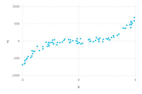
In addition to training data, we should also have testing data. What we really aim for is high performance on the testing data, not the training data. It's actually a bit wasteful to do training on just 70–90% of data so there are better ways to estimate testing (out-of-sample) performance. Many ways to make training agree with testing also exist.
However, the more data one has, the less impact the data split would have. In this example, we have infinite data from a simulator so it doesn't matter at all. In cutting-edge AI research, it is common to use games as simulators of very complex data.
xtest, ytest = simulate(50)We transform the data so that it lies between 0 and 1 and complies with the formatting that Flux uses. This transformation is just for the optimization to work. We can transform back to the original scale as long as we record the parameters used. In general, however, transformations are effectively part of the model (assumptions) and should be thought about carefully in that context.
function prepare(x, xmin, xmax)
	# xmin is minimum of original vector. Minimum becomes 0.
	# xmax is maximum of the resulting vector. Maximum becomes 1.
	x = (x .- xmin) ./ xmax
	# Float32 uses less precise numbers and memory.
	x = convert.(Float32, x)
	# Vector of size n need to be a Matrix of size (1, n).
	# Flux takes arrays where the last dimension
	# tells how many observations there is.
	x = reshape(x, 1, length(x))
	return x
end
Now we apply the transformation.
# "Parameters" needed for the [0,1]-scaling.
xmin = minimum(x)
xmax = maximum(x .- xmin)
ymin = minimum(y)
ymax = maximum(y .- ymin)

# f refers to Flux.
xf = prepare(x, xmin, xmax)
yf = prepare(y, ymin, ymax)
# Note that test data needs to be transformed using
# parameters from the training data.
xftest = prepare(xtest, xmin, xmax)
yftest = prepare(ytest, ymin, ymax)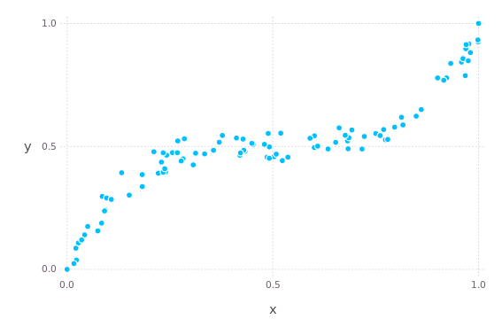
Using the framework of generalized linear models, we could add some terms to a simple linear model to make the model more flexible. You could also use many simple models for many short intervals where the patterns are still simple. Finally, you would use some link functions to relate values from different distibutions. You could call this "wide learning".
So, in deep learning models, you instead nest those simple linear models so that linear models feed to other linear models. More generally, the model is some kind of combination of linear algebra and simple functions, forming a network architecture. Importantly, neural networks have activation functions (like link functions) that keep the values around 0–1 to improve optimization. The absolute values in the hidden layers have no meaning, only the result of the complete network is relevant.
We'll use the following simple model structure with 22 parameters between 3 layers.
model = Chain(
	# "Dense" layers connect all values to each other
	# by multiplying (weights) and adding to (bias) to all inputs.
	Dense(1 => 3, σ),
	# σ is an S-shaped "activation" function that
	# maps all values between 0 and 1.
	Dense(3 => 3, σ),
	Dense(3 => 1)
)
To train the parameters, we need an evaluation function that measures the quality of each candidate model. In this example, we prefer models that minimize the mean of squared differences between the predicted y and the true value of y in the training data.
loss(model, x, y) = Flux.mse(model(x), y)In order to search the optimal parameters, we need an optimization algorithm. Here we use Adam which is a kind of gradient (rate of change) descent method. The details don't matter much until there are problems that cannot be solved by other means. Sometimes tuning, changing, or combining optimizers can help.
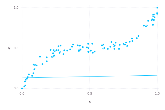
optimizer = Flux.setup(Adam(), model)Currently the model makes predictions like this (the line).
plot(
	layer(x = xf, y = yf, Geom.point),
	layer(x = xf, y = model(xf), Geom.line)
)
Next we train the model.
function train(data, tests, model, loss, optimizer; epochs, batchsize)
	# Independent copies that can be modified instead of the arguments.
	model = deepcopy(model)
	optimizer = deepcopy(optimizer)

	# Often all observations cannot be fed into
	# the model at once. Instead, you can divide the data
	# into batches of certain size.
	dataloader = Flux.DataLoader(data, batchsize = batchsize)

	# Measure prediction errors every now and then
	# during training so that we can check them later.
	mse_epoch = []
	mse_train = []
	mse_test = []

	# Epoch is used to mean one pass over the whole dataset.
	# It depends on many things how many epochs you might need.
	# Often you can just run until some condition is not fulfilled.
	# Instead of a fixed for-loop, you would use a conditional while-loop.
	for e in 1:epochs

		# For every batch of the dataset.
		for (x, y) in dataloader
			# Calculate the changes in loss that happen
			# when each parameter is changed a tiny bit one-by-one.
			# This gives a direction towards which to change
			# the parameters next in order to decrease the loss.
			gradients = Flux.gradient(loss, model, x, y)
			# Update the model parameters according to
			# the optimization rule that uses the gradients.
			optimizer, model = Flux.update!(
				optimizer,
				model,
				gradients[1]
			)
		end

		if e % 1000 == 0
			push!(mse_epoch, e)
			# At this moment of training,
			# compute the prediction error on
			# both training and testing data.
			push!(mse_train, loss(model, data...))
			push!(mse_test, loss(model, tests...))
		end

	end
	return (
		model = m,
		evals = DataFrame(
			epoch = mse_epoch,
			train = mse_train,
			test = mse_test
		)
	)
end
Calling the train-function would then look like this.
trained_model, evals = train(
	(xf, yf),
	(xftest, yftest),
	model,
	loss,
	optimizer,
	epochs = 100_000,
	batchsize = 2^6
)
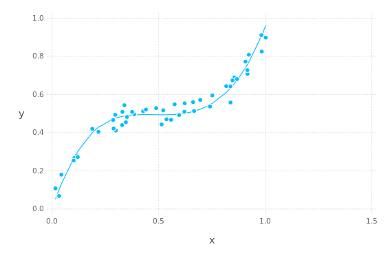
If we now repeat the plot from above, we see that the model fits the training data smoothly.
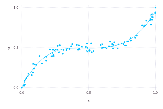
The same thing on test data.
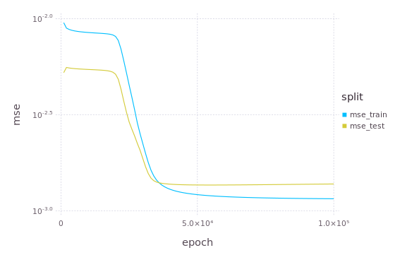
Finally, this is how the loss (mean squared error) decreased during training.
The trained model can be now used like any other function in Julia to approximate the simulator or data generating process from x to y.