The Basic Idea of Probabilistic Programming in Julia Turing

using Distributions, Turing, Gadfly, Chain
import Cairo, Fontconfig, DataFrames as DF

Let’s say we have some data like this.

function simulate(n::Int)
	# Draw n samples from Normal(10, 4) and save as "a".
	a = rand(Normal(10, 4), n)
	b = rand(Normal(0, 2), n)
	# @. macro "broadcasts" all operations in the expression.
	# None of the functions work on collections originally
	# but with the dot-syntax they do.
	c = @. rand(Normal(2.0*a + 3.5*b, 5))
	d = rand(Poisson(10), n)
	e = @. rand(Normal(4 + 4.0*c + (-2.0)*d + 3.0*a, 3))
	# Concatenate vectors horizontally to make a matrix. 
	return hcat(a,b,c,d,e)
end

Now, we simply want to model the data generating system/mechanism and update our uncertainty based on observations from the system.

Most importantly, we want to stay at a lower level of abstraction than usual. Instead of fitting some ready-made models or algoritms designed by others, we want to describe our assumptions about the data generating system freely and explicitly using probability distributions and general-purpose programming. This way the assumptions made in the model are clear to everyone and tailor-made for our data and goals. We then use a general inference algorithm that updates the probability distributions in the model.

So we measure some data from the simulator.

# "simulate" returns a matrix.
data = simulate(100)
# It's often easy to work with dataframes, a common
# data structure in data analysis. It's simply a table where
# observations are on rows and variables on columns.
df = DF.DataFrame(data, [:a, :b, :c, :d, :e])
# When multiple packages export the same name,
# you need to "import" the module and access the name from there.

It’s often useful to rescale variables by subtracting the mean and dividing by the standard deviation, or in other words, by Z-scoring. Model is then written for the standardized variables. Results can be always transformed back to the original scales as long as the parameters have been saved. One of the variables has count values which we’ll just model directly with the Poisson distribution.

zscore(x) = (x .- mean(x)) ./ std(x)
dezscore(z, mn, sd) = (z .* sd) .+ mn

summaries = describe(df, :all)

# Transformed dataset.
dfs = DF.transform(df, [:a, :b, :c, :e] .=> zscore; renamecols = false)

In a real analysis, we of course wouldn’t know the true data generating system. But we can always write a simulator that describes our assumptions about the true system. And then we can use this simulator to assist in writing the model which will be very similar to the simulator.

Usually some variables are always observed and we don’t model how they are generated. In this example we make the model fully generative so that it doesn’t except any variables to be observed. Infact we can easily run the model without any observations and updated it with partly missing observations.

So let’s define the model using Turing.

@model function model(a, b, c, d, e)
	n = length(a)

	# Simulation: a = rand(Normal(10, 4), n)
	ma ~ Normal(0, 2) # Prior uncertainty about mean of a.
	sa ~ Exponential(10) # Prior uncertainty about dispersion of a.
	for i in 1:n
		# "a" in observation "i" is assumed to have 
		# a Gaussian distribution.
		# However this is relevant only when "a" is missing. 
		a[i] ~ Normal(ma, sa)
	end

	# Simulation: b = rand(Normal(0, 2), n)
	mb ~ Normal(0, 2)
	sb ~ Exponential(10)
	for i in 1:n
		b[i] ~ Normal(mb, sb)
	end
		
	# Simulation: d = rand(Poisson(10), n)
	l ~ Exponential(10)
	for i in 1:n
		d[i] ~ Poisson(l)
	end
		
	# Simulation: c = @. rand(Normal(2.0*a + 3.5*b, 5))
	αc ~ Normal(0, 2) # Prior uncertainty about intercept of equation.
	βc ~ filldist(Normal(0, 2), 2) # Two coefficients from two distributions.
	sc ~ Exponential(10)
	for i in 1:n
		mc = αc + βc[1]*a[i] + βc[2]*b[i]
		c[i] ~ Normal(mc, sc)
	end
	
	# Simulation: e = @. rand(Normal(4 + 4.0*c + (-2.0)*d + 3.0*a, 3))
	αe ~ Normal(0, 2)
	βe ~ filldist(Normal(0, 2), 3)
	se ~ Exponential(10)
	for i in 1:n
		me = αe + βe[1]*a[i] + βe[2]*c[i] + βe[3]*d[i]
		e[i] ~ Normal(me, se)
	end
end
# The need to use for-loops in this example is a technical detail of Turing. 

Then we can condition this model of the observed, transformed vectors.

condmodel = model(dfs.a, dfs.b, dfs.c, dfs.d, dfs.e)

And then we apply a general inference algorithm (an adaptive Hamiltonian Monte Carlo sampler, specifically the No U-Turn Sampler, NUTS) to update the prior uncertainty based on the observations. In other words, the conditioned model above is the posterior distribution and NUTS is a method to get samples from this distribution.

# You need to run the sampling process multiple times to see that 
# they agree (chains converge to the same distribution).
posterior = sample(condmodel, NUTS(), MCMCThreads(), 1000, 4)
# With "MCMCThreads" this would be done simultaneously on 4 threads
# as long as julia was set up with 4 threads (julia -t 4).

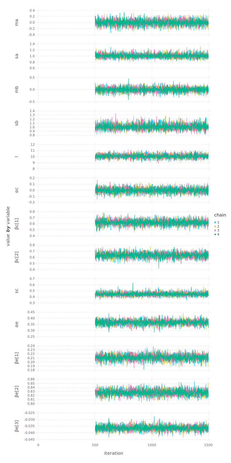
Let’s look at the samples sequentially. You should see that the chains are “tracing” the same distribution randomly.

Now we can use the model and the posterior distributions (samples) to predict new values. And not just some averages but distributions with full uncertainty properly included. We can condition the model again on any observed values to predict distributions of the other variables. Or since the model is fully generative, we can set all variables missing and predict new values for all of them (and transform back to the original scales to apply somewhere).

postpreds = predict(
	model([missing], [missing], [missing], [missing], [missing]),
	posterior
)

Note that we skipped many critically important steps and this would not be a good workflow for solving real problems. Hopefully, however, the basic idea of probabilistic programming is now slightly clearer.