How Probabilistic Programming Allows Automatic Causal Inference

A sidenote on my Julia environment: I use the Julia packages listed below. (Also note that the easiest way to install Julia itself is via juliaup by running the shell script curl -fsSL https://install.julialang.org | sh on Linux distributions or Mac.

# Probabilistic programming metapackage.
using Turing
# Data visualization.
using CairoMakie, AlgebraOfGraphics
using AlgebraOfGraphics: density
# Tabular data processing.
using DataFrames
using DataFramesMeta: @transform
# Chaining functions.
using Chain: @chain
# Identity matrix to construct a variance-covariance matrix.
using LinearAlgebra: I

Sidenote II: Julia and the whole ecosystem around data analysis is still not mature. You might want to use Stan or something for more serious things.

Confounding

Let’s say x is a cause of y, and z is a cause of them both. Given some theory of causal inference, you know that z is a confounder so if you wanted to estimate the effect of x on y, you’d need to adjust for z with some method.

Instead of adjustments, let’s just think about how all of the variables are generated. Then let’s generate data for some inputs of interest and compare them. This is actually equivalent to using a method from causal inference like the parametric g-formula.

First make some simple data for this scenario:

function make_confounding(n)
	
	μz = zeros(n)
	σz = 2	
	z = rand.(Normal.(μz, σz))

	βx = [2, -0.5]
	# [a b] without commas is a 2-column matrix.
	# z causes x.
	μx = [ones(n) z] * βx
	σx = 1		
	x = rand(MvNormal(μx, σx*I))
	
	βy = [1, 1.5, 1.5]
	# x and z cause y.
	μy = [ones(n) x z] * βy
	σy = 1
	y = rand(MvNormal(μy, σy*I))

	return (y, z, x)
end

y, z, x = make_confounding(100)
# Often you want to use Z-scored variables in models 
# but I skip it here for simplicity.

Get a sense of the data space by visualizing.

function plot_xzy(x, z, y)
	
	xyplot = data((x = x, y = y)) * 
		mapping(:x, :y) *
		visual(Scatter)
	
	zxplot = data((z = z, x = x)) * 
		mapping(:z, :x) *
		visual(Scatter)
	
	zyplot = data((z = z, y = y)) * 
		mapping(:z, :y) *
		visual(Scatter)

	f = Figure(size = (400 * (8/4), 400))
	draw!(f[1,1], xyplot)
	draw!(f[1,2], zxplot)
	draw!(f[1,3], zyplot)

	f
end

plot_xzy(x, z, y)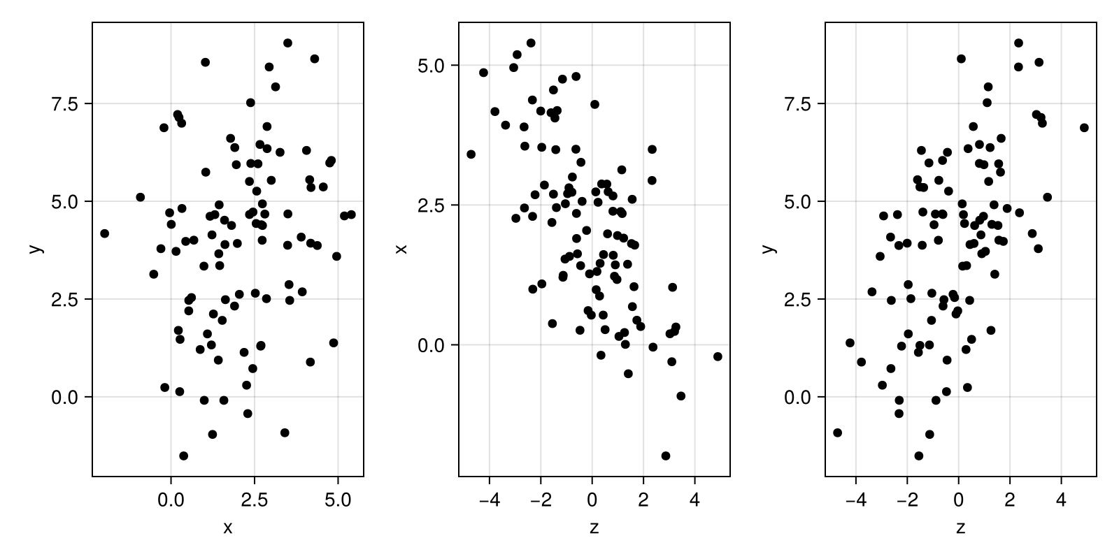

So, we write a generative model of this data assuming z is a common cause. The comments show how the data was generated — note how it differs from the model for that data. The model should look like the generator (simulator).

@model function model_confounding(n, z)

	# We don't model z at all. This is standard in regression models.
	# z is considered fixed and the model doesn't run without it.
	# μz = zeros(n)
	# σz = 2	
	# z = rand.(Normal.(μz, σz))
	
	βx ~ filldist(Normal(0, 2), 2) # βx = [2, -0.5]
	μx = [ones(n) z] * βx # μx = [ones(n) z] * βx		
	σx ~ truncated(Normal(0, 10), 0, Inf) # σx = 1
	x ~ MvNormal(μx, σx * I) # x = rand(MvNormal(μx, σx*I))
	
	βy ~ filldist(Normal(0, 2), 3) # βy = [1, 1.5, 1.5]
	μy = [ones(n) x z] * βy # μy = [ones(n) x z] * βy
	σy ~ truncated(Normal(0, 10), 0, Inf) # σy = 1
	y ~ MvNormal(μy, σy * I) # y = rand(MvNormal(μy, σy*I))

	# In DynamicPPL returning is only for saving generated quantities.
	# return (y, z, x)
end

Condition the generative model on observations of x, z, and y and get the posterior distributions of the parameters.

postmc = sample(
	# In DynamicPPL, you can use "| (..., )" to condition on observations.
	# Function arguments do the same thing but here I use the arguments
	# for fixed values that the model cannot run without whereas
	# x and y can be predicted given z.
	model_confounding(100, z) | (x = x, y = y), 
	NUTS(),
	1000
)

For simplicity, I only sampled one chain. Below you can see how the chain is mixing and what the posterior probabilities look like.

function plot_chains(c)
	p = names(c, :parameters)
	
	chain_mapping = mapping(
		p .=> "value", 
		color = :chain => nonnumeric, 
		row = dims(1) => renamer(p)
	)
	
	p1 = data(c) * mapping(:iteration) * chain_mapping * visual(Lines)
	p2 = data(c) * chain_mapping * density()
	
	f = Figure(size = (1000 * (6/9), 1000))
	draw!(f[1, 1], p1; facet=(linkyaxes=:none, ))
	draw!(
		f[1, 2], p2; 
		facet=(linkxaxes=:none, ), 
		axis = (xticks = -0.5:0.5:2, )
	)
	return f
end

plot_chains(postmc)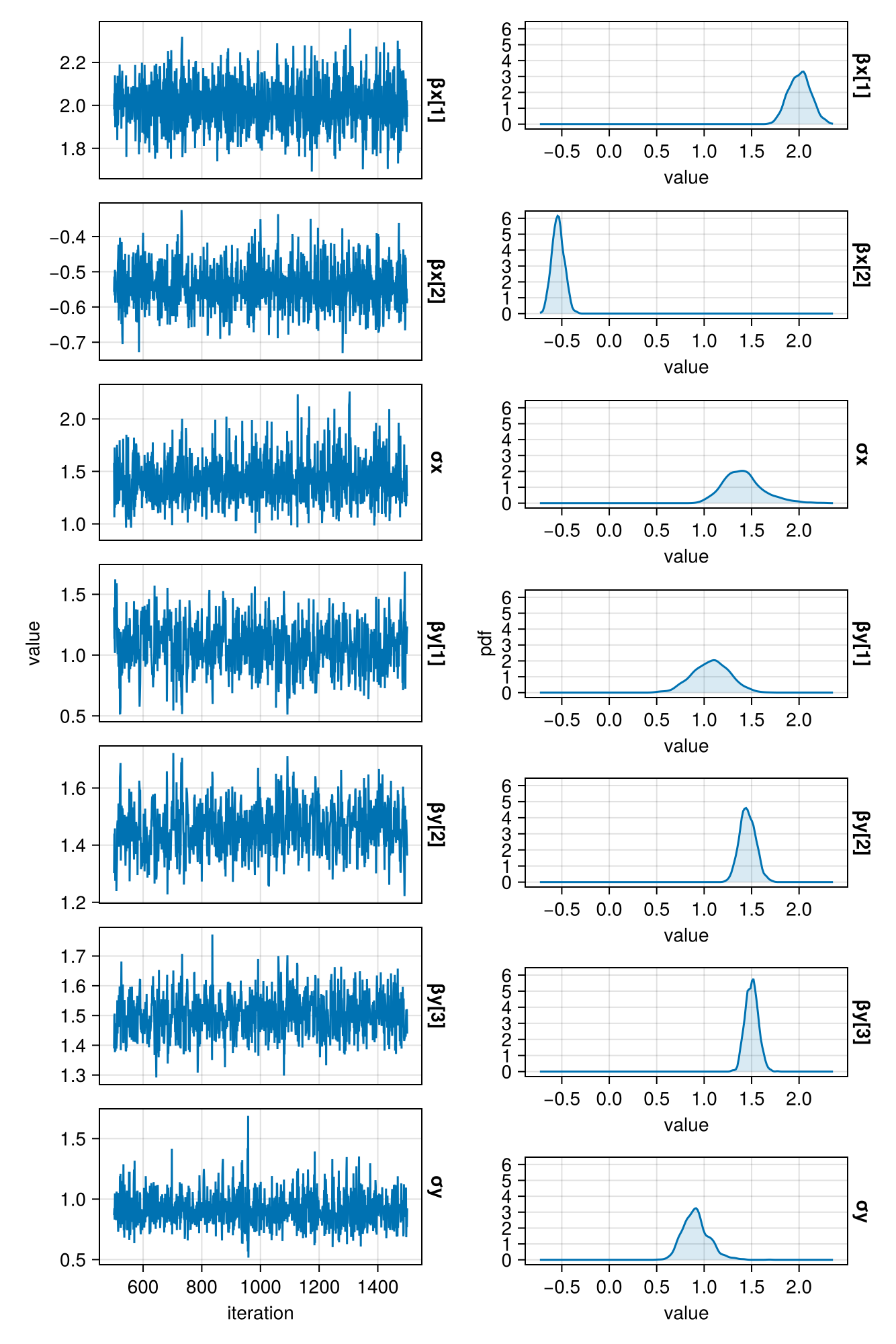

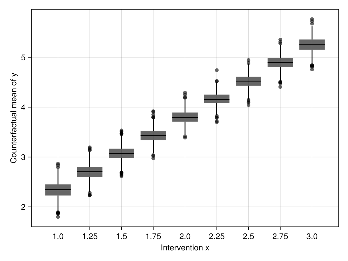
Now, to estimate the effect of x on y, we can predict y given a fixed x and each observed z, and then take the mean of the predicted y. This gives a counterfactual mean of y under the intervention x. Finally, we could compare the means to get some measure of effect.

Follow the comments for this slightly tricky process.

# "let ... end" creates a local hard scope. This means that variables created
# within the scope are not accessible outside the scope (prevents "pollution"). 
let
	predict_mean(intervention::Pair) = @chain begin
		# Instantiate model with observed values of z.
		model_confounding(100, z)
		# Condition the model on counterfactual observations
		# where x is set to some value for everyone.
		condition(x = last(intervention))
		# Predict y for everyone (y[1...100]) for
		# all parameter samples. Predictions are always
		# distributions in fully probabilistic models.
		predict(postmc)
		DataFrame
		select(Not(:chain))
		# Add a label of the intervention to the result.
		# Note that @transform is a macro from DataFramesMeta.jl.
		@transform :intervention = first(intervention)
		# Calculate the mean of predicted y of everyone (y[1...100]).
		stack(Not([:iteration, :intervention]))
		groupby([:iteration, :intervention])
		combine(:value => mean)
	end

	# I label the intervention [1, 1, ..., 1] for everyone as 1.
	# By the way, if you use the observed values as "the intervention"
	# that's sometimes called the natural course intervention.
	x_interventions = Dict(1:0.25:3 .=> [repeat([i], 100) for i in 1:0.25:3])	

	# mapreduce applies (maps) the first function to the collection
	# in the third argument and then reduces the resulting vector
	# into a single object using the second function.
	cfmeans = mapreduce(predict_mean, vcat, x_interventions)

	# Visualize using AlgebraOfGraphics.
	p = data(cfmeans) * 
		mapping(
			:intervention => nonnumeric => "Intervention x", 
			:value_mean => "Counterfactual mean of y"
		) *
		visual(BoxPlot)
	
	draw(p)
end

The boxes show the posterior probability distribution of the mean of predicted y given the counterfactual inputs x and z. Comparisons of any two interventions could be made in a similar way.

Mediation

Now, let’s make z a mediator on the path from x to y instead. I just use a, b, and c in the code — the effect of a on c is partly mediated by b.

The data generator is basically the same.

function make_mediation(n)
	
	μa = zeros(n)
	σa = 2	
	a = rand.(Normal.(μa, σa))

	βb = [2, -0.5]
	# [a b] without commas is a 2-column matrix.
	# a causes b.
	μb = [ones(n) a] * βb
	σb = 1		
	b = rand(MvNormal(μb, σb*I))
	
	βc = [1, 1.5, 1.5]
	# a and b cause c.
	μc = [ones(n) a b] * βc
	σc = 1
	c = rand(MvNormal(μc, σc*I))

	return (c, b, a)
end

c, b, a = make_mediation(100)
plot_abc(a, b, c)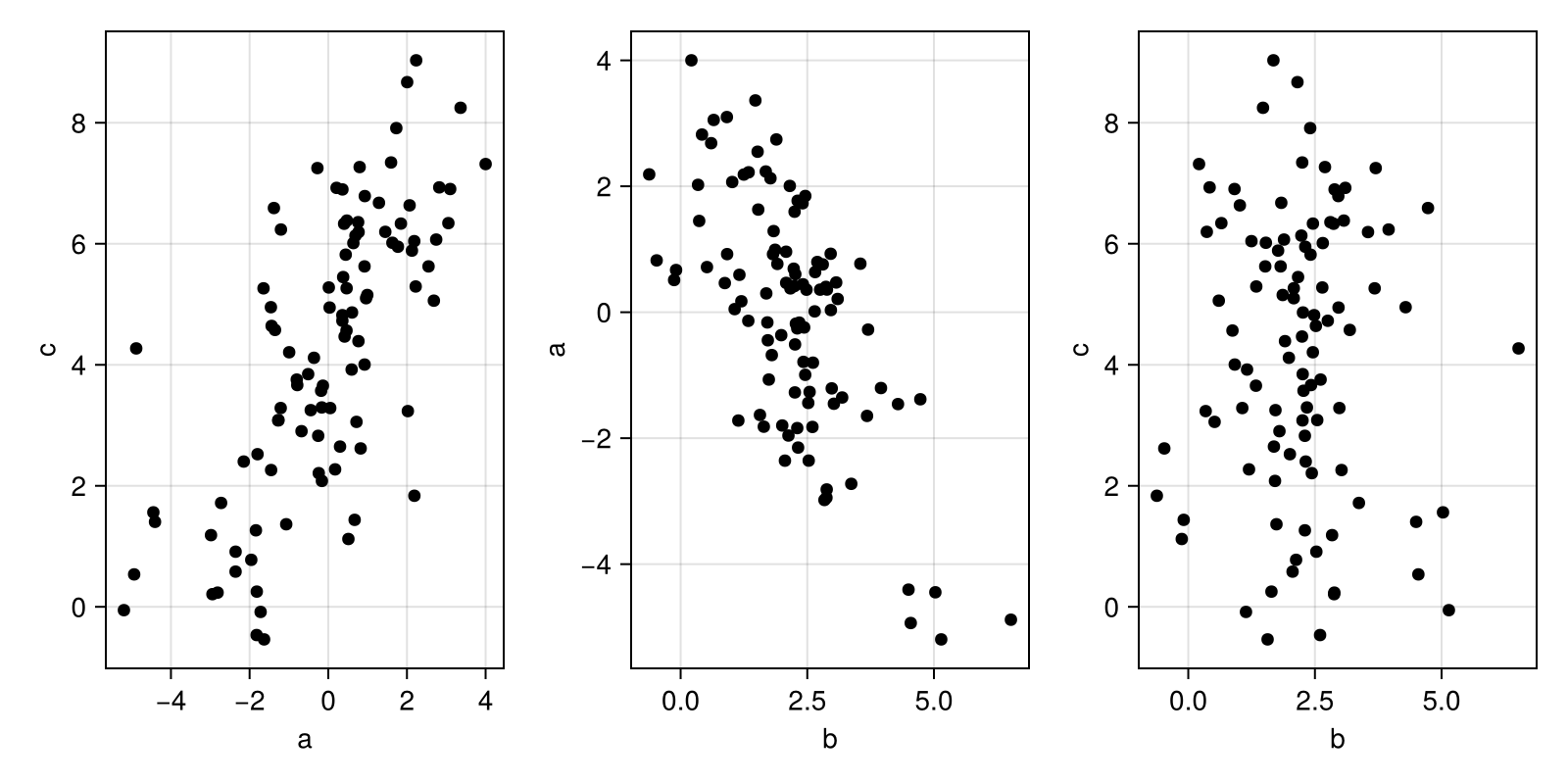

According to causal inference, you shouldn’t include b in your model since the total effect of a on c is already exchangeable without adjustments. But in a generative model, you just continue thinking about how the data is generated. You can include the mediator b in the model if you model it correctly as being caused by a and causing c.

@model function model_mediation(n, a)

	# We don't model a at all. This is standard in regression.
	# a is considered fixed so that the model doesn't run without it.
	# μa = zeros(n)
	# σa = 2	
	# a = rand.(Normal.(μa, σa))
	
	βb ~ filldist(Normal(0, 2), 2) # βb = [2, -0.5]
	μb = [ones(n) a] * βb # μx = [ones(n) a] * βb
	σb ~ truncated(Normal(0, 10), 0, Inf) # σb = 1
	b ~ MvNormal(μb, σb * I) # x = rand(MvNormal(μb, σb*I))
	
	βc ~ filldist(Normal(0, 2), 3) # βc = [1, 1.5, 1.5]
	μc = [ones(n) a b] * βc # μc = [ones(n) a b] * βc
	σc ~ truncated(Normal(0, 10), 0, Inf) # σc = 1
	c ~ MvNormal(μc, σc * I) # y = rand(MvNormal(μc, σc*I))

	# In DynamicPPL returning is only for saving generated quantities.
	# return (c, b, a)
end

Get the posterior distributions again.

postmm = sample(
	model_mediation(100, a) | (b = b, c = c), 
	NUTS(),
	1000
)
plot_chains(postmm)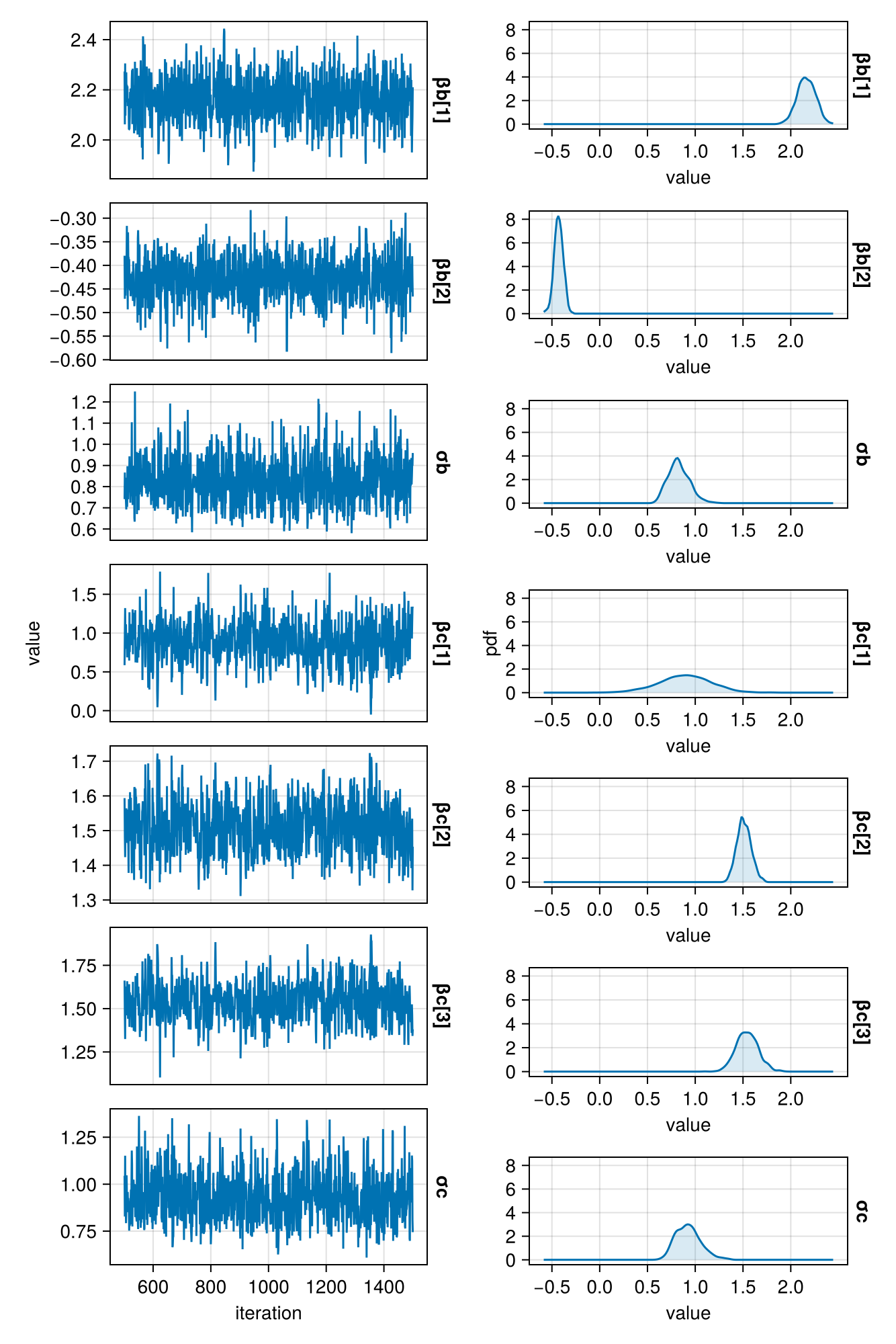

Again, we make predictions of c given some fixed counterfactual values of a for everyone. In this case, we first need to predict b and then use both a and predicted b to predict c. Thankfully, the predict method in Turing does it so we can use pretty much the same code as before.

let	
	predict_mean(intervention::Pair) = @chain begin
			# Now the intervention vector goes to the argument.
			model_mediation(100, last(intervention))
			predict(postmm)
			DataFrame
			# The predictions also include the b[1...100].
			# But we are interested in the mean of c.
			select(:iteration, Between("c[1]", "c[100]"))
			# Add label of the intervention to the result.
			@transform :intervention = first(intervention)
			# Calculate the mean.
			stack(Not([:iteration, :intervention]))
			groupby([:iteration, :intervention])
			combine(:value => mean)
	end

	# The code below is the same as above.
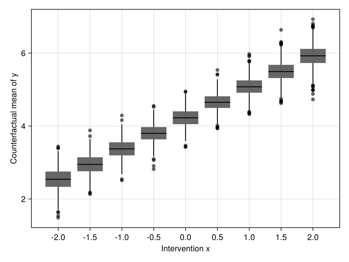
	a_interventions = Dict(-2:0.5:2 .=> [repeat([i], 100) for i in -2:0.5:2])
	cfmeans = mapreduce(predict_mean, vcat, a_interventions)

	p = data(cfmeans) * 
		mapping(
			:intervention => nonnumeric => "Intervention x", 
			:value_mean => "Counterfactual mean of y"
		) *
		visual(BoxPlot)
	
	draw(p)
end